Usage
Examples
Illustrative example
To use pyETC in a project:
>>> import os
>>> from pyETC.pyETC import etc

>>> # load ETC with a config file and the COLIBRI caracteristics
>>> COLIBRI_ETC=etc(configFile=os.getenv('pyETC_DIR')+'/pyETC/configFiles/example.hjson',
         name_telescope='COLIBRI')

>>> # Execute
>>> COLIBRI_ETC.sim()
It will display the following information in the terminal:
Information about the simulation:
---------------------------------
Compute the SNR reached when observing the object during 1 exposure(s) of 5.00 seconds
Object: /data/calspec//bd02d3375_stis_001.txt

Information about Passband:
----------------------------
Filter: COLIBRI r
Cut_on: 5495 angstroms
Effective wavelength: 6199 angstroms
Cut_off: 6895 angstroms

Information about Local conditions:
----------------------------
Site: OAN_Ratir_X1.5
Seeing at zenith: 1.00
Elevation: 41.90 degrees
Airmass: 1.50
Moon age: 7.00

MEAN EFFICENCIES:
------------------
Obscuration: 0.80
Telescope: 0.57 (+obs: 0.46)
Instrument: 0.67
Optics (tel+inst): 0.38  (+obs: 0.30)
Filter: 0.85
Atmosphere: 0.89
Camera: 0.91
System: 0.38 (+obs: 0.30)

Zeropoint: 24.12 (AB mag)


A magnitude (AB system) of 9.81 in r band within a total exposure time of 5.00 seconds splited in 1 exposure(s), implies a total SNR of :

	 - Integrated SNR over 1 pixels: 1375.86


A magnitude (AB system) of 9.81 in r band within a total exposure time of 5.00 seconds splited in 1 exposure(s), implies a SNR for the central pixel of of :

	 - SNR of the central pixel: 1429.23


Full well capacity of 1 pixel: 350000.00 (electrons)

--------- One pixel only------------------

Photo-electrons created: central pix for 1 exposure(s) of 5.00 sec
	by:
	- Object:         2042807.68   (electrons)
	- Sky:                 42.44   (electrons)
	- Readout:              8.00   (electrons)
	- Dark current:         0.01   (electrons)
	- Digitization:         0.43   (electrons)

SNR: -central pixel: 1429.23

Total of electrons collected in the central pixel during an exposure time of 5 seconds: 2042858.56
--> Central pixel saturated: number of electrons > Full well Capacity


--------- Integrated over 1 pixels------------------

Photo-electrons created: brightest pix |  total of 1 pixels, 1 exposure(s) of 5.00 sec
	by:
	- Object:         2042807.68   |   1893093.96   (electrons)
	- Sky:                 42.44   |        42.44   (electrons)
	- Readout:              8.00   |         8.00   (electrons)
	- Dark current:         0.01   |         0.01   (electrons)
	- Digitization:         0.43   |         0.43   (electrons)

SNR: -central pixel: 1429.23
     -integrated over 1 pixels: 1375.86

Total of electrons collected in the brightest pixel during an exposure time of 5 seconds: 2042858.56
--> Brightest pixel saturated: number of electrons > Full well Capacity
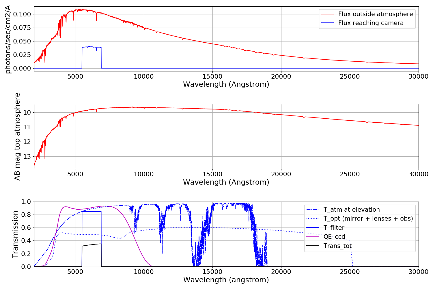
As well as a summary plot:
Compute the SNR for a given magnitude and exposure time
We keep using COLIBRI telescope and let’s say we want to compute the SNR reached for a magnitude of 18 (AB) in a single exposure of 20s in the i band.
>>> COLIBRI_ETC.information['etc_type'] = 'snr'
>>> COLIBRI_ETC.information['object_type'] = 'magnitude'
>>> COLIBRI_ETC.information['object_magnitude'] = 18
>>> COLIBRI_ETC.information['exptime'] = 20
>>> COLIBRI_ETC.information['filter_band'] = 'i'
>>> COLIBRI_ETC.sim()
It will also display information and plots but we do not show them here. If you just want the SNR, you can get it through:
>>> COLIBRI_ETC.information['SNR']
49.92
Compute the limiting magnitude for a given SNR and exposure time
We keep using COLIBRI telescope and this time we want to compute the limiting magnitude in the J band for a SNR of 10 and a single exposure of 30s. We need to use the NIR channel, which is named CAGIRE in the hjson file.
>>> COLIBRI_ETC.information['etc_type'] = 'mag'
>>> COLIBRI_ETC.information['SNR'] = 10
>>> COLIBRI_ETC.information['exptime'] = 30
>>> COLIBRI_ETC.information['channel'] = 'CAGIRE'
>>> COLIBRI_ETC.information['filter_band'] = 'J'

>>> COLIBRI_ETC.sim()
It will also display information and plots but we do not show them here. If you just want the magnitude, you can get it through:
>>> COLIBRI_ETC.information['mag']
19.13
Add new Telescope
The telescopes are stored in pyETC/telescope_database/ in a hjson format. This file contains all caracteristics of the telescope and its environment you do not need to modify for different observations. (Size of the mirrors, number ad type of lenses, mirrors…, sky background, atmosphere transmission, cameras caracteristics,…).
An example is seen below with the default.hjson. The hjson file is composed of 4 parts: the local conditions, main telescope characteristics, optical design and cameras characteristics.
Local conditions
This part contains information related to the observational site: sky brightness and atmosphere transmission. The sky brigthness is loaded from a file stored in pyETC/local_conditions/sky_brightness/, where the magnitude per arcsec^2 is given for different filter bands and at different moon age. A moon age of 0 and 14 correspond to a new moon and a full moon respectively. For instance the file corresponding to the sky brightness at the Observatorio Astronomico Nacional is:
# Sky brightness for Observatorio Astronomico Nacional, Mexico.
# OAN data : http://www.astroscu.unam.mx/rmaa/RMxAC..28/PDF/RMxAC..28_mtapia.pdf
Band eff_wvl 0 14
U 3500 21.5 19.3
B 4400 22.3 19.8
V 5500 21.4 19.7
R 6400 20.7 19.6
I 7900 19.2 18.4
J 12600 16.5 16.5
H 16125 14.1 14.1
K 22000 14.9 14.9
The atmospheric transmission can be either loaded from a file or computed if extinction data are available. In the example below, it is loaded from the file OAN_atm_trans located in pyETC/local_conditions/atmosphere/.
Telescope
Optical design
Cameras
#-------- LOCAL CONDITIONS  ---------------------#
# File containing sky brightness.
# File must be in pyETC/local_conditions/sky_brightness/
"sky_site": OAN

# Wheter the atmospheric transmission is loaded from a file or computed using
# the extinction: "file" / "data"
"atmosphere_type": file

# Name of the file for atmospheric transmission.
# File must be in pyETC/local_conditions/atmosphere/
"atm_file": OAN_atm_trans

#-------- TELESCOPE -----------------------------#
# M1 diameter (in m)
"D_M1": 2

# M2 diameter (in m)
"D_M2": 0.7

# Factor to take into account additional obscuration such as the spider arms.
# It just multiplies D_M2 with this factor
"M2_factor": 1.0

# focal_length (in meters)
"focal_length": {
              "VIS1": 8.124
              "VIS2": 8.124
          }

# FWHM of the optics in arcsec, same for each band
"Fwhm_psf_opt": 0.4

#-------- OPTICAL DESIGN  -----------------------------#
# Modelisation of the telescope and instrument. There are 2 options:

# If detailed == 1: number of mirrors, lenses, dichroics must be defined as
# well as the the filer transmission curves and camera quantum efficiency
# If detailed == 0: will load a global throughput curve

"detailed_trans": 1

# The following is required only if detailed == 1.

# Folder containing the filters transmission of the telescope.
# Has to be in pyETC/transmissions/filters

"filter_folder": default

# Set up the type and number of optical elements in the telescope and each
# intrument channel.
# Note that the keywords used for defining the instrument channels are free
# to chose (here: VIS1, VIS2). However they must be the same as for the camera
# properties below.
# 'telescope' contains all optical elements common for all channels
# For each type of element (i.e 'mirrors', 'lenses'...) must correspond a folder
# in pyETC/transmissions/
# These folders contain files in which the transmission are given.
# For instance here we have one lense N-BaK4 and the file must be
# pyETC/transmissions/lenses/N-BaK4.txt
# You can add your own files and folders.

"optical_design": {

       "telescope": {
           "mirrors": {"Al_OHP_unam": 3}
           "lenses": {"N-BaK4": 1}
           "coating": {"template_tel": 4}
           "dichroics": {"template_tel": 1}
           }

       "VIS1": {
           "coating": {"template_vis": 2}
           "dichroics": {"template_vis": 1}
           "windows": {"template_vis": 1}
           }

       "VIS2": {
           "lenses": {"internal_trans_tot": 1}
           "coating": {"template_vis": 2}
           "dichroics": {"template_vis": 1}
           "windows": {"template_vis": 1}
           }
}

#-------- CAMERAS --------------------------------#
# Characteristics of cameras for the different channels.
# The keywords VIS1 and VIS2 defining the instrument channels must be the same
# as the ones used for the optical design.

"cameras":{

       "VIS1": {
           # Folder must be in pyETC/transmissions/detectors/
           "camera_type": e2v231_84

           # File must be in pyETC/transmissions/detectors/'camera_type'/
           "sensor": bv

           # Number of photocells on X axis
           "Nphotocell_X": 4096

           # Number of photocells on Y axis
           "Nphotocell_Y": 4096

           # Size of 1 photocell on X axis (in meters)
           "Photocell_SizeX": 15e-6

           # Size of 1 photocell on Y axis (in meters)
           "Photocell_SizeY": 15e-6

           # Time required to read all the photocells (in s)
           "ReadoutTime": 6

           # Full well capacity of one photocell (in e-)
           "FWC": 350000

           # Readout Noise (in e-/photocell)
           "RN": 8.0

           # Dark current for one photocell (in e-/photocell/s)
           "DC": 0.001

           # e- to ADU conversion factor
           "gain": 1.5

           # Number of bits for the camera
           "bits": 16}

       "VIS2": {
           # Folder must be in pyETC/transmissions/detectors/
           "camera_type": e2v231_84

           # File must be in pyETC/transmissions/detectors/'camera_type'/
           "sensor": dd_SI_100C

           # Number of photocells on X axis
           "Nphotocell_X": 4096

           # Number of photocells on Y axis
           "Nphotocell_Y": 4096

           # Size of 1 photocell on X axis (in meters)
           "Photocell_SizeX": 15e-6

           # Size of 1 photocell on Y axis (in meters)
           "Photocell_SizeY": 15e-6

           # Time required to read all the photocells (in s)
           "ReadoutTime": 6

           # Full well capacity of one photocell (in e-)
           "FWC": 350000

           # Readout Noise (in e-/photocell)
           "RN": 8.0

           # Dark current for one photocell (in e-/photocell/s)
           "DC": 0.001

           # e- to ADU conversion factor
           "gain": 1.5

           # Number of bits for the camera
           "bits": 16}
}